Gaussian Graphical Model for Expression Arrays

When genomics data is profiled with microarrays, such as with mRNA arrays, miRNA arrays, or methylation arrays, Gaussian graphical models should be used to estimate the network structures. Similar workflows as presented in last section can be applied to fitting Gaussian Markov Networks to data that approximately follows a multivariate Gaussian distribution.

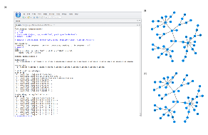
Here, we show an example on fitting simulated Gaussian multivariate data with GGM (Gaussian graphical model). Output of the code snippets below is shown in Figure S2.

> library(XMRF)
> n = 300
> p = 50
   
# Simulate a scale-free network from multivariate Gaussian data
> sim <- XMRF.Sim(n=n, p=p, model="GGM", graph.type="scale-free")
> simDat <- sim$X
   
# Run Gaussian Model and display the results
> ggm.fit <- XMRF(simDat, method="GGM", N=100, stability="STAR", nlams=10, beta=0.05, th=1e-4)
> ml = plotNet(sim$B)
> ml = plot(ggm.fit, mylayout=ml)

Figure S2: Results of fitting a Gaussian graphical model on simulated multivariate Guassian data. (A) Screen shot of the commands and output of fitting GGM model over a path of 10 regularization parameters from R studio. Simulated true network (B) and the estimated network from XMRF (C).