Poisson Graphical Model for NGS data

Count data generated by next generation sequencing (NGS) is a good example of why parametric families of Markov Networks beyond Gaussian graphical models are needed. This read count data is highly skewed and has large spikes at zero so that standardization to a Gaussian distribution is impossible. Here, we demonstrate through a real example how to process NGS data so that we can use Poisson family graphical models to learn the network structure. Our processing pipeline is given in (Allen and Liu, 2012) and encoded in the processSeq function of the package.

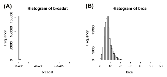
The level 3 RNA-Seq (UNC Illumina HiSeq RNASeqV2) data consisting of 445 breast invasive carcinoma (BRCA) patients from the Cancer Genome Atlas (TCGA) project was obtained. The set of 353 genes with somatic mutations listed in the Catalogue of Somatic Mutations in Cancer (COSMIC) were further extracted. The data was prepared and stored as the brcadata data object included in the package. The values in this data object are the normalized read counts (RSEM) obtained from TCGA data download portal, representing the mRNA expression profiles of the genes. The data matrix is of dimension pxn. Figure S1 shows that the data is more appropriate for Poisson family graphical models after being preprocessed with the processSeq function as given in the following code snippets:

> library(XMRF)
> data('brcadata')
> brca = t(processSeq(t(brcadat), PercentGenes=1))

Figure S1: Distribution of TCGA BRCA RNA-Seq data before (A) and after (B) preprocessing. The latter gives a distribution more appropriate for Poisson family graphical models.

To estimate the underlying network structure of the count-valued data, XMRF implements four different models from the Poisson family graphical models: regular Poisson graphical model (PGM) that only permits negative conditional dependencies, truncated Poisson (TPGM), sub-linear Poisson (SPGM), and local Poisson (LPGM) (Allen and Liu, 2013). The latter three models are variants of the Poisson family that relax restrictions as imposed in a regular Poisson model, resulting in both positive and negative conditional dependencies (Yang et al., 2013b). TPGM should be used if one wants to truncate the large counts observed in NGS dataset. Alternatively, SPGM implements a sub-linear truncation for the NGS data which gives a softer reduction on large counts. LPGM is a faster algorithm that approximates the Markov Network while preserving both positive and negative relationship (Allen and Liu, 2013).

In practice, we choose LPGM since it is the fastest and most flexible way to capture both positive and negative dependencies:

> p = nrow(brca)
> n = ncol(brca)
> lambda = lambdaMax(t(brca)) * sqrt(log(p)/n) * 0.1

# Run Local Poisson Graphical Model (LPGM)
> lpgm.fit <- XMRF(brca, method="LPGM", N=1, lambda.path=lambda)